Harmony Amid Chaos
Galois tables of GF(p²): three theorems on the symmetry between twin tables, and two measures, Arnold's and our own, of how randomly the logarithms are spread.
Abstract
We provide a brief but intuitive study on the subjects from which Galois Fields have emerged and split our study up into two categories: harmony and chaos. Specifically, we study finite fields with \(p^2\) elements where \(p\) is prime. Such a finite field can be defined through a \(p \times p\) logarithm table. The Harmony Section is where we provide three proofs about the overall symmetry and structure of the Galois Field as well as several observations about the order within a given table. In the Chaos Section we make two attempts to analyze the tables, the first by methods used by Vladimir Arnold as well as (what we believe is) an improvement of his method, the second by statistical analysis of the Galois Fields at \(p = 17\), the highest prime value we were able to generate Galois Fields of size \(p^2\) for.
Introduction
A Galois Field is a field with a finite number of elements, which belongs to a subset of “the most fundamental mathematical objects” and supplies a foundation for “all other mathematical structures and models” (Arnold, 2011, p. 1).
Perhaps the best place to begin is with an easily understood, but nonetheless complex, mathematical object, the prime numbers:
which of course form that set of integers greater than zero which only have two divisors (these being \(1\) and \(p\)). But much lesser known than the prime numbers are the set of elements which form what is known as a field.
A field is closed under the operations of addition and multiplication (with associative, commutative, and distributive properties) such that every element has an additive inverse and every nonzero element has a multiplicative inverse.
Consider a prime number, \(p\); a field can be formed by the residues modulo \(p\). For instance, the simplest field, \(p = 2\). I should like to introduce the notation \(GF(p)\), taking \(p = 2\), to mean the field
A simple check ensures that this set is closed under addition and multiplication and contains the inverses it needs (note that since we are adding and multiplying elements of \(\Z /2\Z \), the operations will be closed):
Therefore, \(GF(2)\) is a field. A similar example and proof can be made for \(GF(3)\) using the same method above. With \(GF(4)\), however, a more tactile approach is needed.
If \(\Z /4\Z = \{0, 1, 2, 3\}\) then the number \(2\) has no inverse, since the residues of \(2x\) equal \(0\) or \(2\). This alone seems to imply that a field with four elements does not exist. But they do; enter the finite field.
Such fields were first introduced in the 1800s by a young mathematician named Évariste Galois. They are part of a subset of fields that are finite and are given the name Galois Fields to honor their creator. Two theorems about finite fields have a direct influence on our study:
- 1.
- The number of elements within a finite field is a prime number, \(p\), raised to some natural number \(n\).
- 2.
- For every such \(p^n\) there is a field with \(p^n\) elements, and any two fields with \(p^n\) elements are isomorphic.
In other words, the notation we introduced above is not precise enough to exhaust the set of finite fields. We shall take \(GF(p^n)\) to mean the Galois Field with \(p^n\) elements (Arnold, 2011, p. 6).
To form a Galois Field with \(p^2\) elements we must consider each element in the field as a linear combination of \(A\)’s and \(1\)’s:
Using this method, it becomes rather easy to generate every single element in a field up to and including additive and multiplicative identities, but it does not give us a good way of telling whether the field is cyclic; in other words, this method tells us almost nothing about the structure of a field. For that, a method of defining the elements must be generated. Take \(GF(2^2)\) into consideration.
Exhausting all possible combinations of \(\alpha \) and \(\beta \) yields the following set:
it may not exactly be clear that this is a field, but the simple test applied above can still be applied:
And here we run into an issue that, on initial inspection, appears to show that \(GF(2^2)\) is not a field: you will notice that \(A^2\), \(A^2 + A\) and \(A^2 + 1\) were not elements in our initial set. However, what we are really beginning to see is that these Galois Fields are behaving much like the imaginary numbers that we are so used to. “\(i^2 = -1\)” is notorious; it is in effect saying, “The square root of negative one does not exist, therefore, let us create this strange value, \(i\), such that \(\sqrt {-1} = i\).” It causes us no pause; we are very used to this strange redefinition of an abstract value. And so, it should cause us no pause here: suppose that \(A^2 = A + 1\), what then?
The problem is alleviated; as we can see, the field is still closed, none of the elements are outside the initial set, and every element has an additive inverse and every nonzero element a multiplicative inverse. You may object to our definition of \(A^2\), noticing the choice is arbitrary. However, if we were to choose \(A^2 = A\), issues would have arisen. For instance, \(A \cdot (A + 1) = A^2 + A = 0\), so neither \(A\) nor \(A + 1\) could have a multiplicative inverse. This is a reasonable objection, but it simply means that \(A^2 = A + 1\) is a far superior choice (in later sections we will go into detail about how to select \(A^2\)).
This may seem insignificant, but it has allowed us also to redefine \(GF(2^2)\) as the powers of \(A\):
Therefore, as an expression of the powers of \(A\), \(GF(2^2) = \{0, A, A^2, A^3\} = \{0, A, A + 1, 1\}\); respectively.
In sum, by defining \(A^2\) we have defined the cyclic group in \(GF(2^2)\). And in general (for \(GF(p^2)\)) we can define these fields with a single recursive operation.
Given a proper choice of \(A^2 = \alpha A + \beta \), such that \(\alpha \) and \(\beta \) are “good” choices, we can express the values of \(A^k\), where \(k \le p^2 - 1\), as the expression
Using this method, we can generate \(GF(2^2)\) as before, but without the hassle of performing algebraic operations (if you like, we recommend trying this out by hand; it may help the reader grasp the operation). This method may seem inferior when dealing with a field with only four elements, but when performing higher order operations during which code will be implemented, the formula is superior.
And it is in this manner that we shall bridge into the topic of this paper, the formulation of the Galois Table, a visual representation of the Galois Field.
The last field we generated was quite simple with only four elements, expressed as \(GF(2^2) = \{0, A, A^2, A^3\} = \{0, A, A + 1, 1\}\), perhaps more clearly as
Consider the table expressing the powers on \(A^k\) akin to a table of logarithms, whereby the elements inside the table represent the power on \(A\) and the indices represent the values \((u_k, v_k)\): the column is \(u_k\) and the row is \(v_k\).
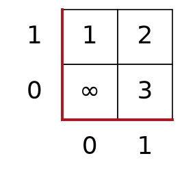
The use of the infinity symbol is based on \(\log (0) = -\infty \): no power of \(A\) is ever \(0\), so the cell for \(0 = 0 \cdot A + 0\) holds no exponent. We write \(\infty \) without a sign, since the elements of a finite field are neither positive nor negative.
Now, choosing the Galois Field from \(p = 2\) is not difficult, as there is only one choice for what \(A^2\) should equal, but for succeeding prime numbers the number of possible fields (choices for \(\alpha \) and \(\beta \)) grows. We wrote code to aid in testing the number of possible logarithm tables for primes under \(200\); this is a sampling of our data:
| \(p\) | Number of \(GF(p^2)\) |
| 2 | 1 |
| 5 | 4 |
| 7 | 8 |
| 17 | 48 |
| 29 | 96 |
| 53 | 432 |
| 89 | 960 |
| 137 | 2816 |
| 173 | 4704 |
| 199 | 4800 |
As the reader can see, the number of tables grows quickly as \(p\) increases. We should note the methodology used to generate tables and why certain values for \(\alpha \) and \(\beta \) are not as “good” as others.
Let \(p = 7\), and suppose that we have used the recursive formulas defined above and a simple nested for loop to generate all possible combinations where \(A^2 = \alpha A + \beta \). Note, there are (by combinations) \(7^2 = 49\) unique combinations for \(\alpha \) and \(\beta \). But, if the reader will look back at the number of possible Galois Fields, they will notice that there are only \(8\). How are we to separate the \(41\) “bad” choices from the \(8\) “good” choices?
Using code, this can be done with Boolean operators. We can use the number of nonzero elements in the field, \(p^2 - 1\), to fix the number of unique elements the recursion must generate: if the recursive formula and the choice of \(\alpha \) and \(\beta \) generate unique values for the first \(p^2 - 1\) (in this case \(48\)) powers, then we keep the table (include it as one of the \(8\)). If, however, the recursive formula and the choice for \(\alpha \) and \(\beta \) repeats before cycling through all \(48\) nonzero elements, then we throw away the table (exclude it from the set of \(8\)).
But this provides no theoretical mathematical framework on which we can judge a table based on the choice of \(A^2\) as good or bad. The method we used beforehand simply iterates the recursive formula \(48\) times with a particular \(\alpha \) and \(\beta \), and tells whether it should be included or excluded based on the uniqueness of the elements produced in the string with length \(48\). But say I were to give the reader \(A^2 = \alpha A + \beta \): what then? Could the reader tell whether it was “good” or “bad” (included or excluded)?
Of course, one could, by hand or by code, repeat the process described above (by hand it would be quite tedious for a large prime number). But if we did not want to go to all that work, or if we did not know how to write code, one of the ways we could tell is whether the equation
(formed by setting \(A^2 = \alpha A + \beta \) equal to zero) has no integer solutions mod \(p\). If it has a solution \(c\), then \(A^2 - \alpha A - \beta = (A - c)(A - c')\) factors, the product of two nonzero elements can be zero, and no field arises; so “good” choices are always among those with no integer solutions.
Notice that this test only rules choices out. There are instances where a choice has no integer solutions but does not generate the table. For instance, in \(p = 5\), there are 4 sets of \(\alpha \) and \(\beta \) that generate the whole field of \(25\) elements; using code these have been identified:
If you set each of these equal to zero, you will find that they have no integer solutions, but you can draw out all the possible combinations for \(\alpha \) and \(\beta \) and you will find that there are \(6\) other choices for \(A^2\) that have no integer solutions. But this is a great improvement given our knowledge of how many possible combinations there are for \(\alpha \) and \(\beta \). In \(p = 5\) there are \(25\) combinations; excluding those with integer solutions, there are 10, only 4 of which end up generating the whole set (those being the ones above).
What separates the two is the order of \(A\). When \(A^2 - \alpha A - \beta \) has no integer solutions, the elements \(\alpha A + \beta \) form the field \(GF(p^2)\), and its nonzero elements form a cyclic group of order \(p^2 - 1\); but \(A\) itself may have smaller order, and then its powers repeat early. A choice is “good” exactly when \(A\) has order \(p^2 - 1\), that is, when \(A^2 - \alpha A - \beta \) is what is called a primitive polynomial. This also explains the counts in the table above: the cyclic group has \(\varphi (p^2 - 1)\) generators, where \(\varphi \) is Euler’s totient function, and each good choice of \(A^2\) is satisfied by exactly two of them (\(A\) and \(A^p\)), so there are
Galois Tables of \(GF(p^2)\) (Lidl & Niederreiter, 1997, ch. 3). For \(p = 7\) this is \(\varphi (48)/2 = 8\).
In sum, we can rid ourselves of the brute force method of iterating every single combination for \(\alpha \) and \(\beta \) to see if the table is filled, and decrease the number of iterations that the program would need to run through.
Using these rules, it is possible to generate tables with an even greater number of elements; the largest tables we generated were from \(p = 17\). In bright green we have highlighted all the prime numbers in the set, and in yellow, we have highlighted the arms of the diagonals (the cells with \(u = v\) or \(u = -v\), where a prime keeps its green). This has been done to note the “twinness” of two tables, which we originally defined using the diagonal arms of the table and the prime numbers within. Below are two twins from \(p = 17\), for \(A^2 = 4A + 3\) and \(A^2 = 13A + 3\), although the reader should note that there are \(48\) total tables using our method of generation.
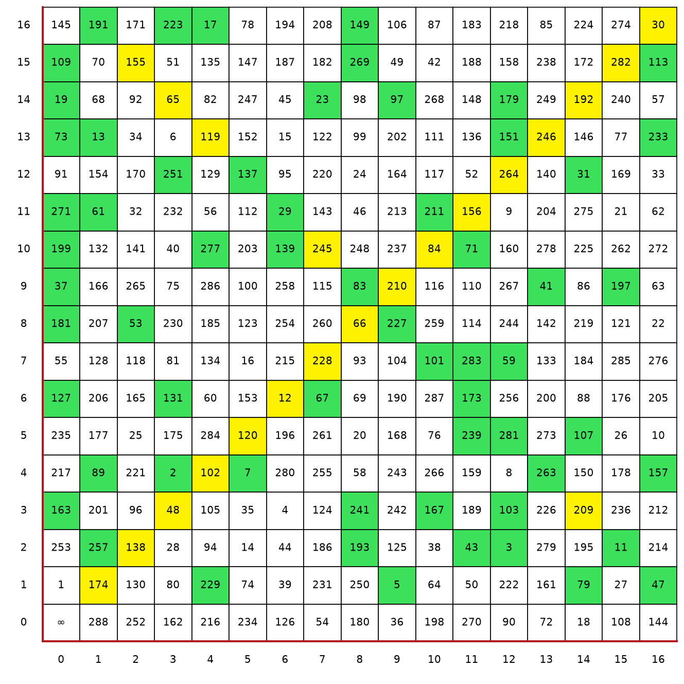
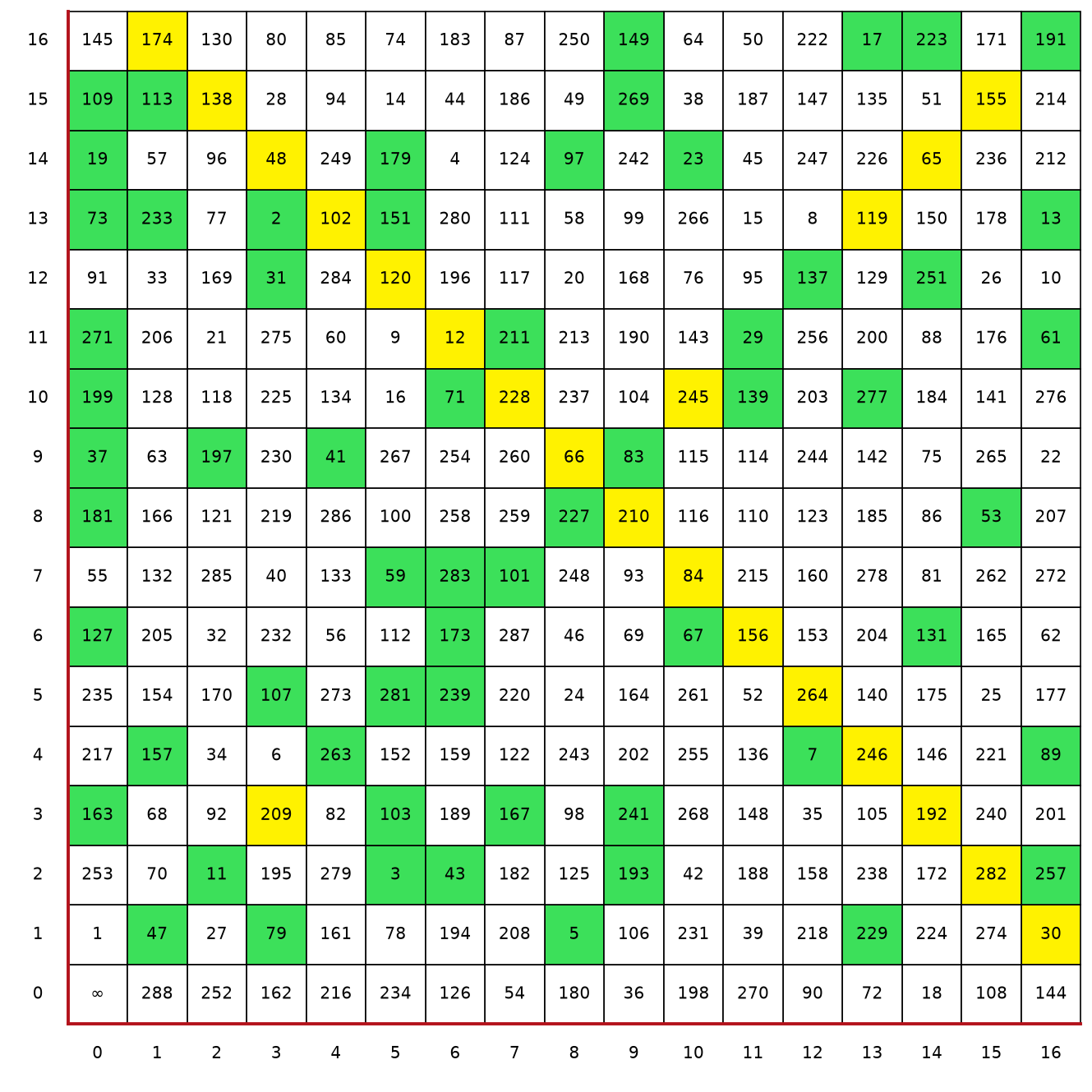
Spend some time gleaning through these two tables, and you will no doubt come to notice two properties.
The first is the “center” of the table. If you have not noticed this, look in the very middle of the diagonal, and subtract elements opposite from one another. So, in Figure 2, subtract \(210 - 66 = 144\) or \(227 - 83 = 144\). This property is reliant on the entry \((17 - 1, 0)\) where \(n = 144\), and can be proven simply for all odd \(p\).
In general, the bottom right corner of the Galois Table is always \(\tfrac 12(p^2 - 1)\). Let \(x = \tfrac 12(p^2 - 1)\). Then \((A^x)^2 = A^{p^2 - 1} = 1\), and the only square roots of \(1\) in a field are \(1\) and \(-1\); since the powers of \(A\) do not repeat before \(A^{p^2 - 1}\), \(A^x \ne 1\), and so \(A^x = -1 = 0 \cdot A + (p - 1)\). And thereby, if we suppose there is some value \(a\) where \(A^a\) is defined by the table, multiplying \(A^a\) by \(A^x\) yields \(-A^a\), and it is precisely this that produces the symmetry defined above: the cells \((u, v)\) and \((-u, -v)\), which (for \(u, v \ne 0\)) sit opposite one another about the center, hold exponents differing by \(\tfrac 12(p^2 - 1)\) modulo \(p^2 - 1\).
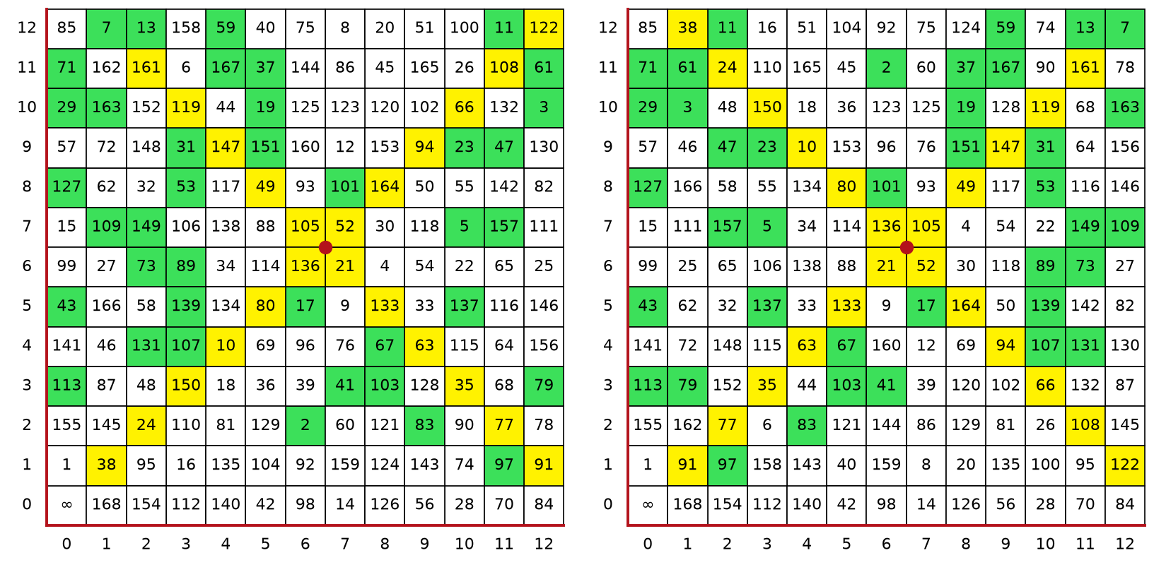
The second property is a little more important in the scheme of our study, which is the difference between two tables, and in general, the twins have a sort of symmetry about each other. The twin of the table for \(A^2 = \alpha A + \beta \) is the table for \(A^2 = -\alpha A + \beta \). The arms of the diagonal rotate about one another when looking between the two tables. The odd values flip across a vertical line through the center of the diagonal, and the even values flip across a similar horizontal line: an odd exponent in cell \((u, v)\) of one table sits in cell \((-u, v)\) of its twin, and an even exponent in cell \((u, v)\) sits in cell \((u, -v)\). (This is Theorem 2 below.) We have included two smaller tables for the reader to examine the property more closely:
Now that the reader has (hopefully) a much clearer grasp of the Galois Fields, we can begin to understand that there are two sorts of emerging categories: one that is ordered, harmony, and another that is far less understood and perhaps more interesting, the property of randomness, chaos.
Harmony
This is a section that is composed of proofs and helps tell us more about the overall harmony within Galois Tables. Throughout, \(p\) is an odd prime; for \(p = 2\) there is only one table, and \(-A = A\).
Theorem 1. If \(A_i^2 = \alpha A_i + \beta \) has no integer solutions mod \(p\), then \(A_k^2 = -\alpha A_k + \beta \) has no integer solutions mod \(p\).
Proof. Let \(A_i^2 = \alpha A_i + \beta \). We take this to mean that \(A_i^2 - \alpha A_i - \beta \) has no integer factors for \(\alpha \) and \(\beta \); such a factorization would imply that \(A_i^2\) is not a “good” choice for \(A^2\).
Suppose for contradiction that \(A_k^2 = -\alpha A_k + \beta \) where \(A_k^2\) has integer factors, which means it is not a “good” choice for \(A^2\). Set it equal to zero, such that
where \(-\beta = c_1 c_2\) and \(\alpha = c_1 + c_2\) for some \(c_1, c_2 \in \Z /p\Z \).
Now set \(A_i^2 = \alpha A_i + \beta \) equal to zero and attempt to find integer solutions based on the factors of \(A_k^2\). Taking the negatives of \(c_1\) and \(c_2\), their sum is \(-\alpha \) and their product is still \(-\beta \), so
and \(A_i^2 - \alpha A_i - \beta = 0\) has the integer solutions \(c_1\) and \(c_2\): a contradiction, since it has no integer solutions.
Therefore, by contradiction, if \(A_i^2 - \alpha A_i - \beta \) has no integer solutions mod \(p\), neither does \(A_k^2 + \alpha A_k - \beta \).
Theorem 2. If \(A_1^n = \alpha ' A_1 + \beta '\), \(A_1^2 = \alpha A_1 + \beta \) and \(A_2^2 = -\alpha A_2 + \beta \), then there is a table where \(A_2^n = -\alpha ' A_2 + \beta '\) if \(n\) is even and \(A_2^n = \alpha ' A_2 - \beta '\) if \(n\) is odd.
Proof by cases. Suppose that \(A_1^n = \alpha ' A_1 + \beta '\), and let \(A_1^2 = \alpha A_1 + \beta \). Put \(A_2 = -A_1\). Then
so \(A_2\) satisfies \(A_2^2 = -\alpha A_2 + \beta \), and its powers make the table for that choice. Since \(A_2^n = (-1)^n A_1^n\):
First case, \(n\) is even:
Second case, \(n\) is odd:
Therefore there is a table where \(A_2^n = -\alpha ' A_2 + \beta '\) if \(n\) is even and \(A_2^n = \alpha ' A_2 - \beta '\) if \(n\) is odd.
Theorem 3. Suppose that \(A_1^2 = \alpha A_1 + \beta \) and \(A_2^2 = -\alpha A_2 + \beta \). If the powers on \(A_1\) generate the Galois Field with \(p^2\) elements, \(\{A_1, A_1^2, A_1^3, \dots , A_1^{p^2 - 1}\}\) where \(A_1^{p^2 - 1} = 1\), then the powers on \(A_2\) also generate the Galois Field with \(p^2\) elements.
Proof. As in the proof of Theorem 2, let \(A_2 = -A_1\), and let \(A_1^{p^2 - 1} = 1\) with no earlier power of \(A_1\) equal to \(1\).
Suppose for contradiction that \(A_2^i = 1\) for some \(0 < i < p^2 - 1\), meaning that the succeeding powers on \(A_2\) repeat elements before wrapping all the way through the nonzero elements of \(GF(p^2)\). Since \(A_2^i = (-1)^i A_1^i\), we split into two cases.
Odd case: suppose \(i\) is odd. Then \(A_1^i = -A_2^i = -1\). We showed above that \(A_1^x = -1\) for \(x = \tfrac 12(p^2 - 1)\), and the powers of \(A_1\) below \(p^2 - 1\) are all different, so \(i = x\). But \(p^2 - 1 = (p - 1)(p + 1)\) is a product of two consecutive even integers, one of which is divisible by \(4\), so \(p^2 - 1\) is divisible by \(8\) and \(x\) is even. This is a contradiction, since \(i\) is odd.
Even case: suppose \(i\) is even. Then \(A_1^i = A_2^i = 1\) with \(0 < i < p^2 - 1\). This is a contradiction, since no power of \(A_1\) before the \((p^2 - 1)\)th equals \(1\).
Therefore, by cases, if the powers on \(A_1\) generate the Galois Field with \(p^2\) elements, then the powers on \(A_2\) also generate the Galois Field with \(p^2\) elements.
Together, Theorems 1 and 3 say that every table has a twin: if \(A^2 = \alpha A + \beta \) is a good choice then so is \(A^2 = -\alpha A + \beta \), and Theorem 2 tells us exactly how the two tables are related.
Chaos
This section is a little more difficult to lay out. Firstly, what do we mean by chaos? Is the nonappearance of order the defining hallmark of chaos? Is the fact that we cannot identify a discernible structure evidence that there is some sort of underlying structure which we are unable to identify, or evidence of no structure whatsoever? These are all very confusing questions, and one of the ways that we have attempted to address them is through coming up with our own method, which is a little different from the method described by Vladimir Arnold.
Arnold’s Conjecture for Equidistribution
The Arnold Method for determining uniformity or equidistribution of a Galois Table relies on dividing the table through a vertical line (which we get to choose); this allows us to specify two areas, the total area, which we shall call \(z\), and the subdivided area, which we shall call \(G\). The fraction \(G/z\) yields the proportion of cells in the section. Then we shall take \(N\) to mean the number of values in the Galois Table less than a value \(m\) which occur in the region \(G\). Then the fraction \(N/m\) is the proportion of \(N\) to the value of \(m\) (Arnold, 2011, p. 17).
Arnold proposes:
(Arnold, 2011, p. 19). And as far as we can tell, this conjecture appears to be true. But his method is only concerned with single tables; during this project, we became more concerned with the variations of all the tables within a field. That is, how does this limit vary with respect to all the choices of \(\alpha \) and \(\beta \)? We have formed a simple table showing this for \(p = 17\) which uses \(m = 145\) in every table and utilizes the first seven columns to divide the table into \(G = 119\) and \(z = 289\). Here is the collected data using Arnold’s Method.
Note that the coordinates represent all of the possible choices of \(\beta \) and \(\alpha \), and the resulting \(\lvert \mathit {Arnold}\rvert = \lvert N/m - G/z\rvert \) is taken by subtracting one side of the equation from the other and then taking the absolute value.
| \((\beta , \alpha )\) | \(\lvert \mathit {Arnold}\rvert \) | \((\beta , \alpha )\) | \(\lvert \mathit {Arnold}\rvert \) |
| \((3, 4)\) | 0.057200811 | \((10, 1)\) | 0.004868154 |
| \((3, 6)\) | 0.025557809 | \((10, 4)\) | 0.022718053 |
| \((3, 7)\) | 0.032454361 | \((10, 5)\) | 0.029614604 |
| \((3, 10)\) | 0.036511156 | \((10, 12)\) | 0.039350913 |
| \((3, 11)\) | 0.029614604 | \((10, 13)\) | 0.008924949 |
| \((3, 13)\) | 0.029614604 | \((10, 16)\) | 0.046247465 |
| \((5, 2)\) | 0.018661258 | \((11, 2)\) | 0.060040568 |
| \((5, 3)\) | 0.011764706 | \((11, 6)\) | 0.036511156 |
| \((5, 5)\) | 0.002028398 | \((11, 8)\) | 0.039350913 |
| \((5, 12)\) | 0.025557809 | \((11, 9)\) | 0.015821501 |
| \((5, 14)\) | 0.039350913 | \((11, 11)\) | 0.050304260 |
| \((5, 15)\) | 0.008924949 | \((11, 15)\) | 0.018661258 |
| \((6, 2)\) | 0.029614604 | \((12, 3)\) | 0.002028398 |
| \((6, 7)\) | 0.057200811 | \((12, 5)\) | 0.022718053 |
| \((6, 8)\) | 0.015821501 | \((12, 8)\) | 0.008924949 |
| \((6, 9)\) | 0.002028398 | \((12, 9)\) | 0.032454361 |
| \((6, 10)\) | 0.015821501 | \((12, 12)\) | 0.004868154 |
| \((6, 15)\) | 0.011764706 | \((12, 14)\) | 0.015821501 |
| \((7, 1)\) | 0.002028398 | \((14, 1)\) | 0.011764706 |
| \((7, 3)\) | 0.004868154 | \((14, 6)\) | 0.087626775 |
| \((7, 4)\) | 0.004868154 | \((14, 7)\) | 0.060040568 |
| \((7, 13)\) | 0.060040568 | \((14, 10)\) | 0.022718053 |
| \((7, 14)\) | 0.008924949 | \((14, 11)\) | 0.004868154 |
| \((7, 16)\) | 0.011764706 | \((14, 16)\) | 0.057200811 |
As you can see, the results are quite close to zero, but there is one issue: the area we have taken into consideration, shown below using a table from \(p = 13\), contains a flaw under Arnold’s Method. This region contains a part of the table which has relative symmetry. This being the diagonals, it would not be an issue if it took only one of the diagonals into consideration, but it does not; as I have outlined a hypothetical area \(G\) in blue below, we can clearly see that both diagonals are included in the calculation:
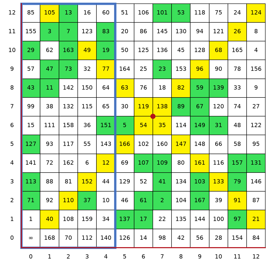
Now to a new observer of these fields, this may not seem to be a large issue, but one must understand that every single table has a twin, and these are identified by the difference between the diagonals (defined at the beginning). So, we can see that at least the most visible symmetry occurs between the diagonals, and then too that if one diagonal possesses even numbers, the other possesses odd values. We argue that this “ruins” the calculation which Arnold proposes to identify the randomness of a table and that if we define a new area, it would be possible to obtain values even closer to zero. So, to solve this issue, we propose a new method, the Morgan Method.
Morgan’s Conjecture for Equidistribution
Following on the tail of Arnold’s Method, the same values will be used, but the area of the table under consideration for uniformity will be slightly different. We will still be comparing the proportion \(G/z\) to the proportion \(N/m\), and their meanings will be the same as above. However, for our area we will be more rigid, always taking into consideration the following area across all tables, under all values of \(p\):
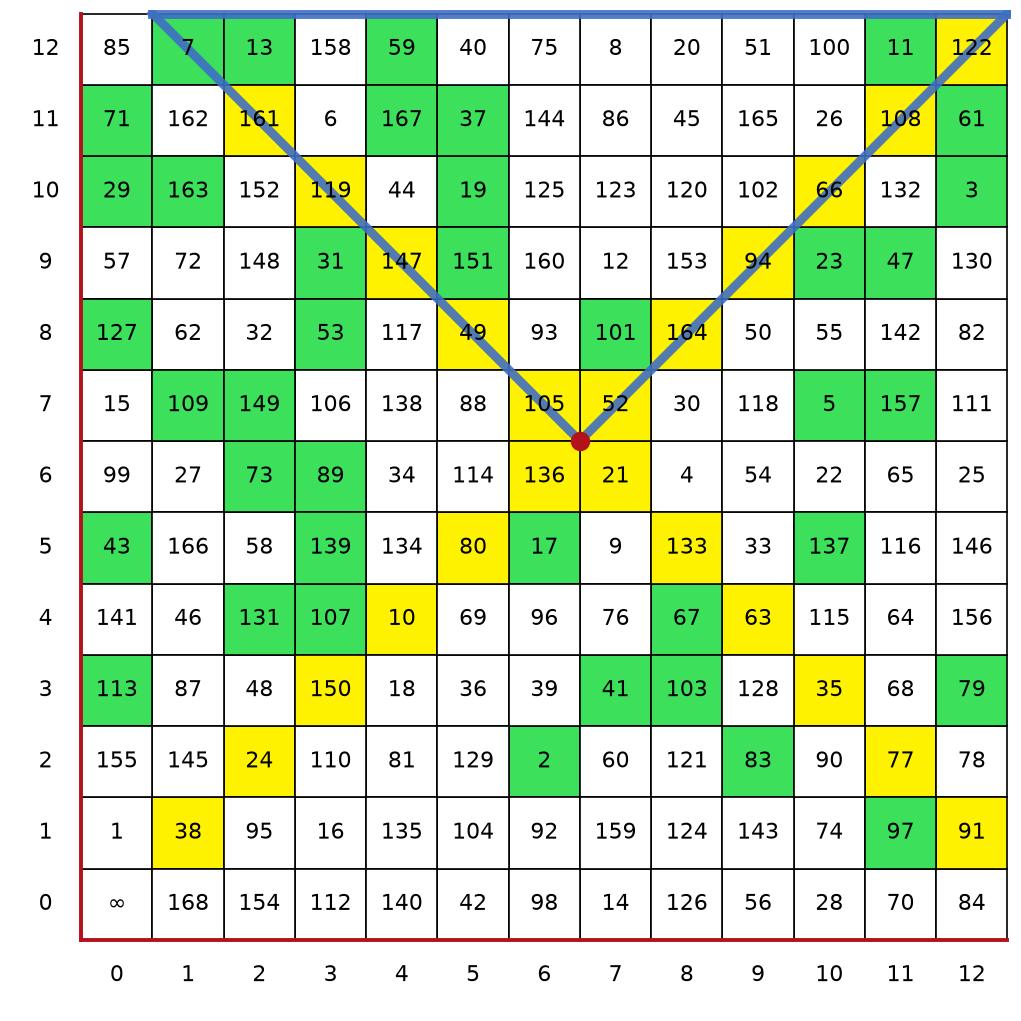
The values under the triangle and inside it: the area of values enclosed inside the arms of the top two diagonals, excluding the diagonal on the right side. Precisely, these are the cells \((u, v)\) in the rows \(v > \tfrac 12(p - 1)\) with \(p - v \le u < v\). All in all, there are \(36\) values, a constant across all tables in \(p = 13\), and an easy way to make the area under consideration uniform for different values of \(p\); in general there are \(\bigl (\tfrac {p-1}{2}\bigr )^2\).
Using \(G = 64\), under \(p = 17\), therefore \(z = 289\), and for \(m\) we will still use \(145\), so we can compare the two methods later on. \(N\), per the definition in Arnold’s Method, will be counted within the new area. Doing so, we obtain the following.
| \((\beta , \alpha )\) | \(\lvert \mathit {Morgan}\rvert \) | \((\beta , \alpha )\) | \(\lvert \mathit {Morgan}\rvert \) |
| \((3, 4)\) | 0.014556735 | \((10, 1)\) | 0.019926023 |
| \((3, 6)\) | 0.019926023 | \((10, 4)\) | 0.006132920 |
| \((3, 7)\) | 0.007660184 | \((10, 5)\) | 0.013029471 |
| \((3, 10)\) | 0.000763632 | \((10, 12)\) | 0.006132920 |
| \((3, 11)\) | 0.006132920 | \((10, 13)\) | 0.006132920 |
| \((3, 13)\) | 0.040615678 | \((10, 16)\) | 0.000763632 |
| \((5, 2)\) | 0.013029471 | \((11, 2)\) | 0.055936046 |
| \((5, 3)\) | 0.035246391 | \((11, 6)\) | 0.019926023 |
| \((5, 5)\) | 0.006132920 | \((11, 8)\) | 0.035246391 |
| \((5, 12)\) | 0.019926023 | \((11, 9)\) | 0.061305333 |
| \((5, 14)\) | 0.000763632 | \((11, 11)\) | 0.075098437 |
| \((5, 15)\) | 0.019926023 | \((11, 15)\) | 0.019926023 |
| \((6, 2)\) | 0.040615678 | \((12, 3)\) | 0.026822575 |
| \((6, 7)\) | 0.040615678 | \((12, 5)\) | 0.033719127 |
| \((6, 8)\) | 0.054408782 | \((12, 8)\) | 0.013029471 |
| \((6, 9)\) | 0.021453287 | \((12, 9)\) | 0.006132920 |
| \((6, 10)\) | 0.026822575 | \((12, 12)\) | 0.014556735 |
| \((6, 15)\) | 0.000763632 | \((12, 14)\) | 0.014556735 |
| \((7, 1)\) | 0.007660184 | \((14, 1)\) | 0.013029471 |
| \((7, 3)\) | 0.007660184 | \((14, 6)\) | 0.062832598 |
| \((7, 4)\) | 0.028349839 | \((14, 7)\) | 0.042142942 |
| \((7, 13)\) | 0.006132920 | \((14, 10)\) | 0.026822575 |
| \((7, 14)\) | 0.013029471 | \((14, 11)\) | 0.028349839 |
| \((7, 16)\) | 0.006132920 | \((14, 16)\) | 0.040615678 |
Is the Morgan Method better than the Arnold Method; that is, does our limit approach zero better than his? Difficult to say; we can only do two things to compare the two methods. The first is statistical: compare the averages, standard deviations, as well as the maximum and minimum value of the methods. The second is a simple difference between each table under both methods using the coordinates of \(\alpha \) and \(\beta \).
| Arnold | Morgan | |
| Average | 0.025946586 | 0.022510241 |
| Standard Dev | 0.019973616 | 0.018074696 |
| Max | 0.087626775 | 0.075098437 |
| Min | 0.002028398 | 0.000763632 |
As the reader can clearly see, the Morgan Method outperforms the Arnold Method slightly under these parameters. The average, standard deviation, max, and min are all lower, implying that the Morgan Method trends closer to zero, perhaps faster than the Arnold Method.
Difference. For the difference, we have simply taken each value for the Arnold Method, \(\lvert \mathit {Arnold}\rvert _{(\beta , \alpha )}\), and subtracted from it \(\lvert \mathit {Morgan}\rvert _{(\beta , \alpha )}\). This can tell us easily which of the values is closest to zero: if \(\lvert \mathit {Arnold}\rvert _{(\beta , \alpha )} - \lvert \mathit {Morgan}\rvert _{(\beta , \alpha )}\) results in a negative value, then for that particular \(\alpha \) and \(\beta \) Arnold is a better method, but if it is positive, then Morgan is better. Here are the results:
| Negatives | Positives |
| -0.011001 | 0.042644 |
| -0.023482 | 0.005632 |
| -0.004105 | 0.024794 |
| -0.011001 | 0.035748 |
| -0.011001 | 0.023482 |
| -0.038587 | 0.005632 |
| -0.019425 | 0.005632 |
| -0.011001 | 0.038587 |
| -0.005632 | 0.016585 |
| -0.002792 | 0.011001 |
| -0.023482 | 0.053908 |
| -0.004105 | 0.005632 |
| -0.015058 | 0.016585 |
| -0.045484 | 0.016585 |
| -0.024794 | 0.033218 |
| -0.001265 | 0.002792 |
| -0.024794 | 0.045484 |
| -0.011001 | 0.004105 |
| -0.004105 | 0.016585 |
| -0.009689 | 0.004105 |
| -0.001265 | 0.026321 |
| -0.004105 | 0.001265 |
| -0.023482 | 0.024794 |
| 0.017898 | |
| 0.016585 | |
As the reader can see, if we take into consideration the difference between the two methods, then the Morgan Method is slightly superior to Arnold’s, be it only by two values: it is closer to zero for 25 of the 48 tables, and Arnold’s for 23.
The statistical and difference based approaches agree, if only narrowly, and we maintain that the Morgan Method is superior to Arnold’s for a further reason, based on observations about the Galois Fields which are not exactly open to statistical criticism: the structure.
Under Arnold’s Method, there are values which are more commonly repeated across the many tables of a Galois Field. For instance, here are four different tables selected from \(p = 13\):
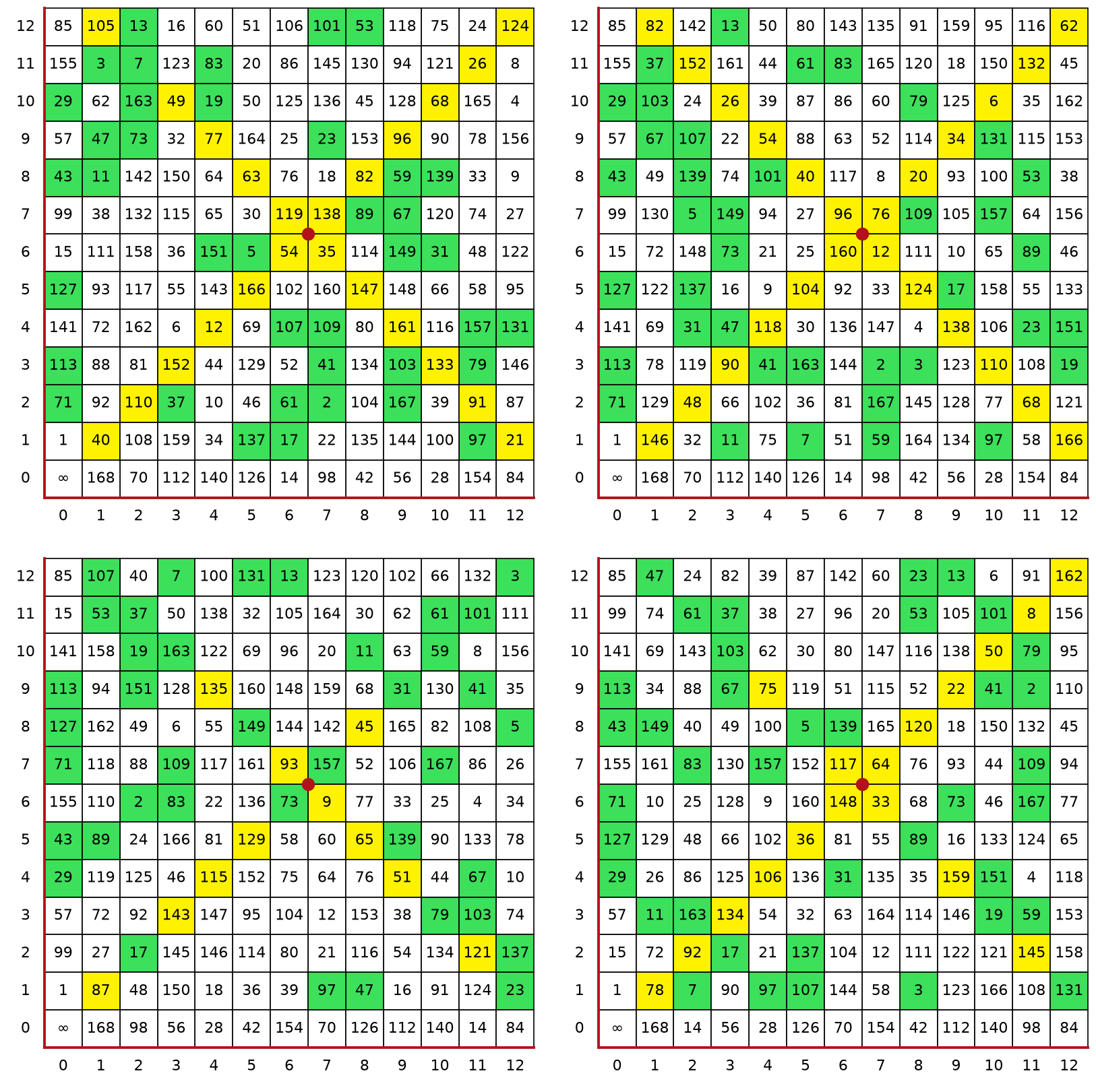
These tables were selected as “randomly” as we could manage, but you will notice that (though this be the case) the tables have a surprising number of similarities.
- 1.
- Along the first column and the bottom row of every table there tend to be values which are the same and which seem to not change, despite changes in many other places in the table. (Every value in the bottom row is a multiple of \(p + 1 = 14\): the bottom row holds the nonzero integers mod \(p\), and these are exactly the powers of \(A^{p+1}\).)
- 2.
- Though we mentioned it at the start of this debate, the diagonals in the table have a surprising amount of predictability within each individual table, and you will recall from the beginning that every table has a “twin.”
- 3.
- Though this seems obvious to state, the \(\infty \) in the bottom left corner is always there.
Given that these similarities exist, we assert that the Morgan Method does not count as many similarities both within individual Galois Tables and within the whole Galois Field as does the Arnold Method, thereby lending the Morgan Method the benefit of having more randomness than the former.
Still, over the course of our project, we were unable to provide a proof for either conjecture, implying that more work needs to be done to discover whether Vladimir Arnold is correct about the equidistribution of the Galois Fields. However, we were able to gather data about how predictable the many tables are within a given field.
The first trial of statistically analyzing the tables was: what do we measure? It was not as simple as taking the standard deviation or average about a table, as this would provide us with no knowledge whatsoever about the Galois Field. So, we began to collect data on individual squares within every single table iteration of a Galois Field.
We collected data from \(p = 11\), \(13\) and \(17\), but for purposes of brevity we are only presenting the data from \(p = 17\), our largest table. Our most influential observation is this: that within individual cells, the values stick around the middle of the range of values. We argue that this implies something approaching equidistribution:
| \((u, v)\) | Mean | Median | \((u, v)\) | Mean | Median | \((u, v)\) | Mean | Median |
| \((1, 1)\) | 144.5 | 144.5 | \((3, 1)\) | 150.5 | 151.0 | \((5, 1)\) | 150.5 | 150.0 |
| \((1, 2)\) | 150.5 | 144.0 | \((3, 2)\) | 132.5 | 135.0 | \((5, 2)\) | 126.5 | 125.0 |
| \((1, 3)\) | 138.5 | 138.0 | \((3, 3)\) | 144.5 | 144.5 | \((5, 3)\) | 138.5 | 121.5 |
| \((1, 4)\) | 144.5 | 139.0 | \((3, 4)\) | 144.5 | 151.5 | \((5, 4)\) | 144.5 | 145.0 |
| \((1, 5)\) | 138.5 | 139.0 | \((3, 5)\) | 150.5 | 167.5 | \((5, 5)\) | 144.5 | 144.5 |
| \((1, 6)\) | 144.5 | 130.5 | \((3, 6)\) | 132.5 | 130.0 | \((5, 6)\) | 132.5 | 130.5 |
| \((1, 7)\) | 144.5 | 133.0 | \((3, 7)\) | 150.5 | 150.5 | \((5, 7)\) | 144.5 | 141.5 |
| \((1, 8)\) | 168.5 | 193.5 | \((3, 8)\) | 150.5 | 146.0 | \((5, 8)\) | 150.5 | 153.0 |
| \((1, 9)\) | 138.5 | 128.0 | \((3, 9)\) | 138.5 | 122.0 | \((5, 9)\) | 138.5 | 124.5 |
| \((1, 10)\) | 144.5 | 128.0 | \((3, 10)\) | 132.5 | 116.0 | \((5, 10)\) | 138.5 | 133.5 |
| \((1, 11)\) | 162.5 | 181.0 | \((3, 11)\) | 150.5 | 152.5 | \((5, 11)\) | 138.5 | 135.5 |
| \((1, 12)\) | 150.5 | 155.5 | \((3, 12)\) | 156.5 | 161.5 | \((5, 12)\) | 138.5 | 133.0 |
| \((1, 13)\) | 132.5 | 128.0 | \((3, 13)\) | 132.5 | 130.5 | \((5, 13)\) | 156.5 | 162.5 |
| \((1, 14)\) | 144.5 | 141.5 | \((3, 14)\) | 138.5 | 130.5 | \((5, 14)\) | 156.5 | 161.0 |
| \((1, 15)\) | 132.5 | 126.5 | \((3, 15)\) | 138.5 | 137.5 | \((5, 15)\) | 132.5 | 116.0 |
| \((1, 16)\) | 132.5 | 128.0 | \((3, 16)\) | 144.5 | 141.0 | \((5, 16)\) | 156.5 | 155.0 |
| \((2, 1)\) | 138.5 | 145.0 | \((4, 1)\) | 144.5 | 150.0 | \((6, 1)\) | 144.5 | 158.5 |
| \((2, 2)\) | 144.5 | 144.5 | \((4, 2)\) | 150.5 | 170.5 | \((6, 2)\) | 156.5 | 165.5 |
| \((2, 3)\) | 156.5 | 154.0 | \((4, 3)\) | 144.5 | 137.5 | \((6, 3)\) | 156.5 | 159.0 |
| \((2, 4)\) | 138.5 | 118.5 | \((4, 4)\) | 144.5 | 144.5 | \((6, 4)\) | 156.5 | 159.5 |
| \((2, 5)\) | 162.5 | 164.0 | \((4, 5)\) | 144.5 | 144.0 | \((6, 5)\) | 156.5 | 158.5 |
| \((2, 6)\) | 132.5 | 123.5 | \((4, 6)\) | 132.5 | 129.5 | \((6, 6)\) | 144.5 | 144.5 |
| \((2, 7)\) | 138.5 | 119.0 | \((4, 7)\) | 138.5 | 137.0 | \((6, 7)\) | 150.5 | 171.0 |
| \((2, 8)\) | 150.5 | 158.0 | \((4, 8)\) | 150.5 | 146.5 | \((6, 8)\) | 150.5 | 163.5 |
| \((2, 9)\) | 144.5 | 143.0 | \((4, 9)\) | 144.5 | 139.5 | \((6, 9)\) | 150.5 | 159.5 |
| \((2, 10)\) | 150.5 | 151.5 | \((4, 10)\) | 138.5 | 134.0 | \((6, 10)\) | 144.5 | 156.5 |
| \((2, 11)\) | 138.5 | 131.0 | \((4, 11)\) | 150.5 | 161.5 | \((6, 11)\) | 138.5 | 134.5 |
| \((2, 12)\) | 144.5 | 141.5 | \((4, 12)\) | 156.5 | 183.5 | \((6, 12)\) | 132.5 | 129.5 |
| \((2, 13)\) | 132.5 | 109.0 | \((4, 13)\) | 132.5 | 120.5 | \((6, 13)\) | 162.5 | 174.0 |
| \((2, 14)\) | 132.5 | 118.5 | \((4, 14)\) | 138.5 | 136.5 | \((6, 14)\) | 144.5 | 151.5 |
| \((2, 15)\) | 138.5 | 137.5 | \((4, 15)\) | 132.5 | 121.5 | \((6, 15)\) | 138.5 | 125.0 |
| \((2, 16)\) | 120.5 | 110.0 | \((4, 16)\) | 120.5 | 102.5 | \((6, 16)\) | 156.5 | 180.5 |
This table seems complicated, and has many rows, but it is not exactly obvious what a given entry of mean and median represents. Consider a value for \((u, v)\), say \((6, 9)\), with a mean of 150.5 and a median of 159.5. This means that across every single one of the 48 tables in \(p = 17\), the value in column \(6\) and row \(9\) has mean 150.5 and median 159.5. The same could be extended to all cells of the table.
After a very brief examination of the table above, you will no doubt find that the values center around \(\tfrac 12 p^2 = 144.5\), the average of all the values \(1, 2, \dots , p^2 - 1\) in a table: the means of the 96 cells lie between 120.5 and 168.5, and the medians, more widely spread, between 102.5 and 193.5. In general, a study in the future might try to verify whether this extends to prime values greater than \(17\).
We assert that this implies a roughly equal or equitable distribution of values within every single table. For if the values within the tables deviate or are weighted too heavily above \(\tfrac 12 p^2\) or below it, then there would be a disparate number of coordinates whose means and medians are quite far away from the midpoint.
This, we believe, is our most valid evidence that the Galois Fields are equidistributed, despite our misgivings about the rudimentary and theoretical mess created by applying measurements like mean and median to something as complex as a finite field.
Future Work
Over the course of eight weeks of study much has been learned, and what has been gained is hopefully established above, but what we must also point out is where we have failed, where we have come short (as these are no doubt the most important) and which mathematicians should continue to study in the future. These are the gaps that we have not been able to fill.
The foremost matters arise in our failure to produce a sufficient proof for Vladimir Arnold’s Conjecture; this said, we did not expect to provide one during our study, given that it would require far longer inquiry. But nor were we truly capable of specifying that it might exist, or that it at least appears to exist. Indeed, the best we can do is a “wholesome maybe.” In our search for statistical randomness we have admittedly come up with crumbs.
One of the initial problems in our study was the code implemented. Though we automated the process of obtaining individual tables within a Galois Field to a far more efficient state than can be done by hand, we were severely limited by our ability to fill tables with the data generated by our code. We started off with the most rudimentary code, that which could generate a single table, followed by more complex iterations till we eventually wrote code which could find every single “viable” table within a Galois Field. This drastically changed our scope of study, since it enabled us to generate tables as large as \(p = 17\), which has \(48\) associated tables, but took roughly five or ten minutes to compute, and then almost two or three hours to convert by clicking and pasting into an Excel file to turn them into the tables the reader has seen above. It was an incredibly painstaking process, and our abilities at writing code were not sufficient to move onto the next prime value.1
What is needed most to further the study is a computer based approach: a code written which not only generates the fields for a prime number, but which also fills and outputs the resulting tables and provides strings of coordinate data associated with each value in the table.
And most importantly, the study of Galois Fields is not nearly complete. We know much about them, about their structure and behavior; we even have whole theorems that pertain to Galois Fields (by way of applying to finite fields). However, juxtaposed with the unknown, our knowledge is the tip of the iceberg.
There are other areas outlined in Vladimir Arnold’s book which we were not able to go into, but which directly relate to the study. For instance, there is a whole subclass called Distribution of Geometric Progressions of Residues, which evaded our study, and another about Projective Structures which has been equally elusive (Arnold, 2011, pp. 37 & 44). From the depths of the structure to the infinite intricacies, what is needed deeply are those willing to study these structures to provide a continuance of Arnold’s work.
Conclusion
The Galois Fields were a daunting task at the start, requiring much mathematical explanation and understanding before we were even able to delve deeply into their harmony and chaos. This said, we were capable of showing several things for ourselves. On Harmony, we have concluded that the structure within a Galois Field is filled with enough order that proofs can be made between tables, but it is also chock full of uncertainties, of Chaos.
The Harmony of a Galois Field is easily defined by the three proofs we have shown:
- 1.
- If \(A_i^2 = \alpha A_i + \beta \) has no integer solutions mod \(p\), then \(A_k^2 = -\alpha A_k + \beta \) has no integer solutions mod \(p\).
- 2.
- If \(A_1^n = \alpha ' A_1 + \beta '\), \(A_1^2 = \alpha A_1 + \beta \) and \(A_2^2 = -\alpha A_2 + \beta \), then there is a table where \(A_2^n = -\alpha ' A_2 + \beta '\) if \(n\) is even and \(A_2^n = \alpha ' A_2 - \beta '\) if \(n\) is odd.
- 3.
- Suppose that \(A_1^2 = \alpha A_1 + \beta \) and \(A_2^2 = -\alpha A_2 + \beta \); then if the powers on \(A_1\) generate the Galois Field with \(p^2\) elements, \(\{A_1, A_1^2, A_1^3, \dots , A_1^{p^2 - 1}\}\) where \(A_1^{p^2 - 1} = 1\), then the powers on \(A_2\) also generate the Galois Field with \(p^2\) elements.
But as for Chaos, that which cannot be proven, we have no proofs to bear. We are empty handed. However, we did collect data.
Data is by far the most important aspect of our study. There was almost nothing out there on Galois Fields that a first-year math student could really understand. There are plenty of complex books on finite fields, but none that are very attainable for a first-year math student. Arnold’s book provided an intuitive way of expressing these fields. What was needed is exploration, and that is what we have provided. Our inquiry has observed the following:
- 1.
- Vladimir Arnold’s Method, and Morgan’s slight improvement, show promise at being proved one day, since they at least appear to grow closer to zero as \(p\) grows.
- 2.
- The fields appear to have the hallmark of randomness, defined by a propensity to be uniformly distributed on a per-cell basis, and this property might lend credence to equidistribution if it cannot be shown by either method above.
It may seem like nothing, given our eight weeks of study, but it is a start. Can it not be hypothesized that we might know more about Galois Fields if they were observed with the same intensity as the prime numbers? People have been hunting for the next largest prime number since the dawn of the byte. If they had had similar vigor for Galois Fields, perhaps we would not be writing this paper. While we have little to show, it is our hope that our study is the first of many that will be conducted one day.
It is to those who would conduct them, to those who would answer the call, that our paper is written. We hope that it provides at least moderate, if not ample, inquiry into Galois Fields and that someone might one day make harmony out of this chaotic branch of Mathematics.
References
-
Arnold, V. I. (2011). Dynamics, statistics and projective geometry of Galois fields. Cambridge: Cambridge University Press.
-
Lidl, R., & Niederreiter, H. (1997). Finite fields (2nd ed.). Cambridge: Cambridge University Press.