Who Gets the Loan?
How much more often are Black, Hispanic and Asian mortgage applicants denied than White applicants in the 2025 HMDA data, and how much of each gap survives controls for income, debt-to-income, loan-to-value, loan type, state and lender? More than half of the Black–White gap remains, but without credit scores that is not proof of discrimination.
Abstract
Using all 2,947,238 home-purchase applications decided in 2025 and reported under the Home Mortgage Disclosure Act, we measure how much more often Black, Hispanic, Asian, American Indian and Pacific Islander applicants are denied than White applicants, and how much of each gap survives once we hold fixed what the public data record about the applicant, the loan, the property, the state and the lender. White applicants were denied 5.9% of the time and Black applicants 16.7%, a raw gap of 10.8 percentage points. Logistic regressions on 2,789,796 complete applications shrink the Black–White gap to 6.2 points, and comparing applicants who applied to the same lender in the same county leaves 4.4 points; the Hispanic gap falls from 6.5 to 3.1 and 1.9 points. The adjusted Black–White gap is positive in every state with enough applications to measure it and at almost every large lender. These adjusted gaps are not estimates of discrimination: the public data omit the credit score, the variable most likely to explain much of the remainder, and a study that observes it finds residual gaps of one to two points.
1 Introduction
A mortgage application ends in one of a handful of ways: the loan is made, the applicant is approved and walks away, the applicant withdraws, or the lender says no. Since 1975 the Home Mortgage Disclosure Act (HMDA, 12 U.S.C. 2801 et seq.) has required most mortgage lenders to report their applications and outcomes, and since the 2018 data the public records have carried far more detail: the debt-to-income ratio, the combined loan-to-value ratio, the property value, the applicant’s age, and up to four reasons for a denial [3, 4]. The public file for 2025 holds 13,543,606 records.
The question we ask of it is simple to state. How much more often are minority applicants denied than White applicants, and how much of that gap remains once we compare applicants who look alike in everything the public data record? The answer matters because the raw gaps are large and widely quoted, and because the step from “adjusted gap” to “discrimination” is one these data cannot take on their own. The Boston Fed study of Munnell, Tootell, Browne and McEneaney [8], which added credit histories and the other variables lenders said they used to the 1990 HMDA records for Boston, set off a long debate about exactly that step [7, 9]. More recently Bhutta, Hizmo and Ringo [2], with confidential credit scores and the recommendations of the automated underwriting systems lenders use, find that observable risk factors explain most of the racial disparities in denials and that unobserved risk factors explain at least part of the residual 1 to 2 percentage point gaps.
We have none of those confidential variables, and we say so throughout. What we can do with the public data is (i) measure the raw gaps precisely, (ii) show how far they shrink as we add each family of controls, from the applicant’s finances to the lender’s identity, (iii) show where the remaining gap is large and where it is small, across income, debt-to-income ratio, state and lender, and (iv) report what lenders themselves say about why they denied. Section 2 describes the data and the sample, Section 3 the statistics, Section 4 the findings and Section 5 what they do and do not mean.
Every number below is computed by the scripts in the entry’s code/ folder. An interactive explorer at https://maths.dsmorgan.com/projects/mortgage-denials/explore lets the reader choose a state, an income band, a debt-to-income band and a loan type, compare raw and adjusted gaps, read the denial reasons, and ask the fitted model for a predicted denial probability.
2 Data
2.1 Source
We use the Snapshot National Loan-Level Dataset for 2025, published by the Federal Financial Institutions Examination Council (FFIEC) with the Consumer Financial Protection Bureau at https://ffiec.cfpb.gov/data-publication/. We downloaded the loan/application register (2025_public_lar_csv.zip) and the transmittal sheet, which names each reporting institution, in October 2026; the server dates the register 23 June 2026. The snapshot is the data as filed at that date; the later one- and three-year datasets fold in resubmissions, so counts may move slightly. The data are public records released by the FFIEC; we attribute them to the FFIEC and the CFPB and change nothing but the selection described below.
The public register is a modified version of what lenders file. Under the Bureau’s disclosure policy [4], the credit score relied on in the decision is among the fields excluded from the public data; the public file keeps only the name of the scoring model (applicant_credit_score_type). It likewise names the automated underwriting system a lender used but not its recommendation. Loan amounts and property values appear as the midpoint of a $10,000 interval (every value in our sample ends in 5,000), the applicant’s age in seven bands, and the debt-to-income ratio in the bins of the FFIEC data dictionary [5]: below 20%, 20 to under 30%, 30 to under 36%, each whole percent from 36 to 49, 50 to 60%, and above 60%. Income is the gross annual income relied on in the decision, in thousands of dollars. There is no loan-to-value field; we use the combined loan-to-value ratio (combined_loan_to_value_ratio).
2.2 Race and ethnicity
Applicants may report up to five races and five ethnicities, for themselves and for a co-applicant. The FFIEC aggregates these into the derived fields derived_race and derived_ethnicity by a published rule [6]: for instance, an applicant who reports White and one minority race is categorized under that minority race, and an application with a White applicant and a minority co-applicant (or the reverse) is categorized as Joint. We turn the two fields into one classification.
Definition 2.1 (Groups). An application is Hispanic if derived_ethnicity is “Hispanic or Latino”, whatever its race. Otherwise it is Joint if either derived field is “Joint”; Not available if the ethnicity is not “Not Hispanic or Latino” or the race is “Race Not Available” or “Free Form Text Only”; and otherwise it takes its derived race: White, Black, Asian, American Indian or Alaska Native (AIAN), Native Hawaiian or Other Pacific Islander (NHPI), or two or more minority races.
So “White” and “Black” below mean non-Hispanic White and non-Hispanic Black. The groups are mutually exclusive and exhaust the sample; White applications are the reference throughout.
2.3 Sample
Table 1 lists the filters in the order we apply them. We keep first-lien home-purchase applications for a principal residence in a one- to four-unit site-built dwelling, excluding business-purpose loans, open-end lines of credit and reverse mortgages (rows reported as “Exempt” on any of these fields fall out here). We keep the three outcomes that record a credit decision on a completed application: action_taken 1 (loan originated), 2 (application approved but not accepted) and 3 (application denied). Withdrawn applications (4), files closed for incompleteness (5), purchased loans (6) and preapproval requests that were denied or approved but not accepted (7, 8) are dropped. We also drop the 171,877 remaining applications made through a preapproval program: their denials are reported under code 7, and 0 of them carry code 3, so keeping them would add approvals without their matching denials. Finally we keep the 50 states and the District of Columbia. All loan types (conventional, FHA, VA and USDA) stay in the sample; loan type is a control.
| Step |
Remaining | Removed | |
| All records in the 2025 public LAR |
13,543,606 | ||
| 1 | Home purchase (loan purpose 1) |
6,687,105 | 6,856,501 |
| 2 | First lien (lien status 1) |
6,439,088 | 248,017 |
| 3 | One to four units, site-built |
5,829,871 | 609,217 |
| 4 | Principal residence (occupancy 1) |
5,144,587 | 685,284 |
| 5 | Not business or commercial purpose |
5,042,212 | 102,375 |
| 6 | Not an open-end line of credit |
5,009,433 | 32,779 |
| 7 | Not a reverse mortgage | 5,009,095 | 338 |
| 8 | Decision made: originated, approved not accepted, or denied | 3,139,327 | 1,869,768 |
| 9 | No preapproval request (preapproval 2) |
2,967,450 | 171,877 |
| 10 | Property in the 50 states or DC |
2,947,238 | 20,212 |
| 11 | Income reported and positive |
2,910,158 | 37,080 |
| 12 | Debt-to-income ratio reported |
2,886,980 | 23,178 |
| 13 | Combined loan-to-value ratio reported |
2,797,216 | 89,764 |
| 14 | Property value reported |
2,789,854 | 7,362 |
| 15 | Applicant age reported |
2,789,796 | 58 |
That leaves 2,947,238 applications with a credit decision, of which 8.9% were denied. For the regressions we also need income, the debt-to-income ratio, the combined loan-to-value ratio, the property value and the applicant’s age; dropping the 157,442 applications (5.3%) that lack one of them leaves 2,789,796 complete cases at 2,399 lenders. The dropped applications are not a random selection: 19.5% of them were denied, against 8.4% of the complete cases, plausibly because a lender that denies early may never record a debt-to-income ratio. Restricting to complete cases lowers every group’s denial rate a little (Table 2) but does not change the ordering of the groups. All figures and tables from here on use the complete cases.
| Group | Applications | Share | Denied (all) | Denied | 95% CI |
| White | 1,452,414 | 52.1% | 6.4% | 5.9% | 5.86–5.94 |
| Black | 205,265 | 7.4% | 17.3% | 16.7% | 16.54–16.87 |
| Hispanic | 396,749 | 14.2% | 12.9% | 12.4% | 12.27–12.48 |
| Asian | 181,872 | 6.5% | 9.4% | 8.9% | 8.77–9.03 |
| American Indian or Alaska Native | 9,568 | 0.3% | 10.8% | 9.8% | 9.23–10.43 |
| Native Hawaiian or Pacific Islander | 3,424 | 0.1% | 12.0% | 11.2% | 10.20–12.32 |
| Two or more minority races | 5,264 | 0.2% | 15.1% | 14.6% | 13.72–15.63 |
| Joint (mixed applicants) | 159,259 | 5.7% | 7.4% | 7.0% | 6.89–7.15 |
| Not available | 375,981 | 13.5% | 10.2% | 9.6% | 9.50–9.69 |
3 Method
Write \(y_i \in \{0,1\}\) for whether application \(i\) was denied, \(g(i)\) for its group, and \(x_i\) for its controls: income (10 bins), the debt-to-income ratio (the 19 reported categories), the combined loan-to-value ratio (7 bins), the loan amount (8 bins), the property value (7 bins), the loan type (conventional, FHA, VA or USDA), the applicant’s age band (7), whether there is a co-applicant, derived sex (4 categories), and whether the loan exceeds the conforming loan limit; in some models also the state and the lender. Every control is categorical, so a model is a set of indicator columns and no functional form is imposed within a bin.
3.1 Raw and adjusted gaps
Definition 3.1 (Raw gap). For a group \(g\) with \(n_g\) applications, let \(\bar y_g = n_g^{-1}\sum _{g(i)=g} y_i\) be its denial rate. The raw gap is \(\bar y_g - \bar y_W\), where \(W\) is White.
We model the probability of denial with a logistic regression,
so that \(\alpha _g - \alpha _W\) is the shift for group \(g\) and \(e^{\alpha _g - \alpha _W}\) its odds ratio: the factor by which the odds of denial, \(p/(1-p)\), are multiplied for a group-\(g\) applicant relative to a White applicant with the same \(x\). Odds ratios are awkward to compare across models because the logit is not collapsible: adding a control that predicts denial moves \(\alpha _g - \alpha _W\) even when the control is independent of group membership. We therefore also report the gap on the probability scale.
Definition 3.2 (Adjusted gap). The adjusted gap for group \(g\) is the average, over the group’s own applications, of the change in predicted denial probability when the group shift is switched off:
This is an average marginal effect taken over the group’s own applicants: what the model says would change for these applications if, with nothing else changed, they were scored like White applications. The first model in our ladder has no controls, and there the adjusted gap is exactly the raw gap.
Lemma 3.3. Let \(\hat \theta \) maximise the logistic likelihood for a design whose columns include an indicator \(d_i \in \{0,1\}\). Then \(\sum _i d_i\bigl (y_i - \Lambda (z_i^\top \hat \theta )\bigr ) = 0\), where \(z_i\) is the full row of the design.
Proof. The log-likelihood is \(\ell (\theta ) = \sum _i [y_i \log \Lambda (z_i^\top \theta ) + (1-y_i)\log (1-\Lambda (z_i^\top \theta ))]\). Since \(\Lambda ' = \Lambda (1-\Lambda )\), its gradient is \(\nabla \ell (\theta ) = \sum _i \bigl (y_i - \Lambda (z_i^\top \theta )\bigr ) z_i\). At an interior maximum the gradient vanishes; the coordinate belonging to \(d\) is the stated sum.
Proposition 3.4. In the model with group indicators only, \(\Lambda (\hat \alpha _g) = \bar y_g\) for every \(g\); hence \(\hat \Delta _g = \bar y_g - \bar y_W\) and the odds ratio is \(\dfrac {\bar y_g/(1-\bar y_g)}{\bar y_W/(1-\bar y_W)}\).
Proof. For \(g \ne W\), Lemma 3.3 applied to the indicator of \(g\) gives \(\sum _{g(i)=g}(y_i - \Lambda (\hat \alpha _g)) = 0\), that is \(\Lambda (\hat \alpha _g) = \bar y_g\). Applied to the constant it gives the sum over all applications; subtracting the other groups leaves the same identity for \(W\). With no controls, Definition 3.2 averages the constant \(\Lambda (\hat \alpha _g) - \Lambda (\hat \alpha _W)\).
3.2 Uncertainty
Applications to the same lender share underwriting rules, staff and systems, so their outcomes are not independent. We estimate (3.1) by maximum likelihood (Newton’s method, with statsmodels) on all complete cases, with no subsampling, and use the cluster-robust (sandwich) covariance with the 2,399 lenders as clusters. The standard error of \(\hat \Delta _g\) follows from the delta method.
Proposition 3.5. Let \(\theta = (\alpha , \beta )\), let \(z_i\) be the design row of application \(i\) and \(z_i^0\) the same row with group \(g\)’s indicator set to zero. Then
and if \(\hat \theta \) is approximately normal with covariance \(V\), then \(\hat \Delta _g\) is approximately normal with variance \(\nabla \Delta _g^\top V\, \nabla \Delta _g\).
Proof. Differentiate Definition 3.2 term by term with the chain rule, using \(\nabla _\theta (z^\top \theta ) = z\); the variance is the delta method applied to the smooth map \(\theta \mapsto \Delta _g(\theta )\).
3.3 A benchmark decomposition
The pooled model (3.1) makes every group share the same \(\beta \). A complementary approach, in the spirit of the Oaxaca–Blinder decomposition, fits the controls to White applications alone and asks how the other groups fare against that benchmark. Let \(\hat \beta _W\) be fitted on White applications with the controls and state indicators, and let \(\hat p_i = \Lambda (x_i^\top \hat \beta _W)\) for every application.
Definition 3.6 (Excess denial rate). The benchmark rate of group \(g\) is \(\bar p_g = n_g^{-1}\sum _{g(i)=g} \hat p_i\) and its excess denial rate is \(E_g = \bar y_g - \bar p_g\).
Proposition 3.7. \(\bar y_g - \bar y_W = (\bar p_g - \bar y_W) + E_g\), and \(E_W = 0\). The White excess is also zero within any state and within any level of any control.
Proof. The identity is \(\bar y_g = \bar p_g + E_g\) rearranged, with \(\bar p_W = \bar y_W - E_W\). Applying Lemma 3.3 to the White fit with the constant, or with the indicator of a state or of a control level, gives \(\sum (y_i - \hat p_i) = 0\) over the White applications concerned, which is \(E_W = 0\) there. (For a reference level, subtract the other levels from the constant’s equation.)
The first term, \(\bar p_g - \bar y_W\), is the part of the raw gap “explained” by the controls: how much more often the White benchmark would deny group \(g\)’s applications because of their incomes, ratios, loans and states. The excess \(E_g\) is the rest. Because it is an average over applications it can be computed for any subset, which is what the state and lender comparisons and the explorer use; in a subset where \(E_W\) is not forced to zero we report \(E_g - E_W\). For a subset with \(n\) applications we attach the standard error \(n^{-1}(\sum \hat p_i(1-\hat p_i))^{1/2}\), the binomial variance under the benchmark. It ignores the estimation error in \(\hat \beta _W\) and the clustering by lender, so it understates the true uncertainty.
3.4 What controls cannot do
The variable we would most like to hold fixed, the credit score, is not in the public data. A linear model makes the consequence explicit.
Proposition 3.8 (Omitted variable). Suppose \(\mathbb {E}[y \mid x, g, s] = x^\top \beta + \gamma \,\mathbf {1}\{g\} + \delta s\) for a credit-risk variable \(s\), and let \(\pi \) be the coefficient on \(\mathbf {1}\{g\}\) in the linear projection of \(s\) on \((x, \mathbf {1}\{g\})\). Then the population least-squares coefficient on \(\mathbf {1}\{g\}\) in the regression of \(y\) on \((x,\mathbf {1}\{g\})\) alone is \(\gamma + \delta \pi \).
Proof. Write \(s = x^\top \rho + \pi \mathbf {1}\{g\} + u\) with \(u\) uncorrelated with \((x,\mathbf {1}\{g\})\). Then \(\mathbb {E}[y\mid x,g,s] = x^\top (\beta + \delta \rho ) + (\gamma + \delta \pi )\mathbf {1}\{g\} + \delta u\), and projecting \(y\) on \((x,\mathbf {1}\{g\})\) removes the uncorrelated term \(\delta u\) (and the error \(y - \mathbb {E}[y\mid x,g,s]\), which is uncorrelated with every function of \((x,g,s)\)).
Higher credit risk raises the denial probability (\(\delta >0\)), and if minority applicants have higher measured risk on average even after conditioning on income and the loan, as [2] report for credit scores, then \(\pi > 0\) and the adjusted gap overstates \(\gamma \). It may also understate it, if some controls are themselves shaped by unequal treatment; we return to both points in Section 5.
3.5 The ladder of models
We estimate five logits, each adding to the last: (1) group indicators only; (2) the applicant and loan controls listed above; (3) state indicators (119 parameters in all); (4) the same model restricted to the 100 largest lenders by applications (1,821,325 applications, 65.3% of the complete cases); and (5) indicators for those 100 lenders, so that the gap is estimated within lender. With 2,399 lenders, a full set of lender indicators in a logit is impractical; model (4) is there so that (5) can be compared on the same applications. As a check that does not depend on the logistic form we also fit linear probability models with the controls and either state indicators or an absorbed indicator for every lender–county pair (222,705 pairs): the latter compares applicants who applied to the same lender for a home in the same county.
4 Results
4.1 Raw gaps
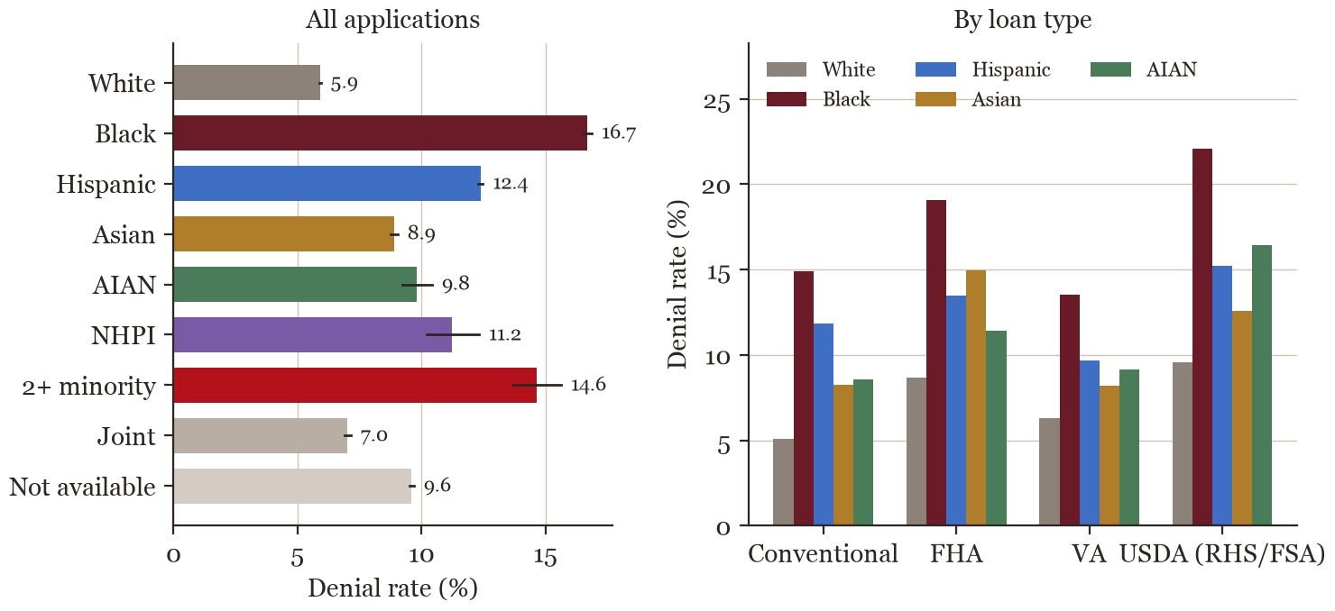
Figure 1 and Table 2 show the raw picture. White applicants were denied 5.9% of the time; Black applicants 16.7%, about 2.8 times as often; Hispanic applicants 12.4%, Asian applicants 8.9%, AIAN applicants 9.8% and NHPI applicants 11.2%. The gaps appear within every loan type. FHA loans, which serve borrowers with smaller down payments and weaker credit, are denied more often (12.4% against 7.0% for conventional loans) and are used more by minority applicants, which is one reason controls matter.
4.2 From raw to adjusted
Table 3 and Figure 2 follow each gap down the ladder. Model (1) reproduces the raw gaps, as Proposition 3.4 says it must. The applicant and loan controls do most of the work: the Black–White gap falls from 10.8 to 6.5 percentage points and the Hispanic–White gap from 6.5 to 3.7. State indicators take off a little more (to 6.2 and 3.1), so the controls and states together account for 42% of the raw Black gap and 51% of the raw Hispanic gap, but only 22% of the smaller Asian gap.
Comparing applications at the same lender narrows the gaps further but does not close them. Among the 100 largest lenders the Black gap is 6.1 points without lender indicators and 5.5 with them; the Asian gap falls from 2.3 to 1.7. Part of each gap is therefore a matter of where applicants apply: lenders with higher denial rates overall receive a larger share of minority applications.
| Group |
|
|
|
|
|
| Black | 10.8 | 6.5 | 6.2 | 6.1 | 5.5 |
| (0.76) | (0.45) | (0.45) | (0.59) | (0.47) | |
| Hispanic | 6.5 | 3.7 | 3.1 | 2.9 | 2.6 |
| (0.60) | (0.30) | (0.28) | (0.33) | (0.26) | |
| Asian | 3.0 | 2.5 | 2.3 | 2.3 | 1.7 |
| (0.28) | (0.17) | (0.17) | (0.21) | (0.30) | |
| AIAN | 3.9 | 2.0 | 2.2 | 2.0 | 2.0 |
| (0.53) | (0.37) | (0.35) | (0.44) | (0.39) | |
| NHPI | 5.3 | 3.1 | 2.9 | 2.5 | 2.5 |
| (0.76) | (0.55) | (0.52) | (0.60) | (0.54) | |
| Applications | 2,789,796 | 2,789,796 | 2,789,796 | 1,821,325 | 1,821,325 |
| Parameters | 9 | 69 | 119 | 119 | 218 |


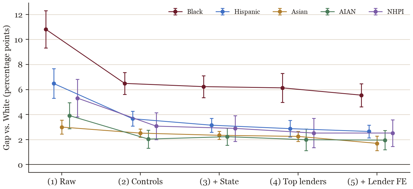
Table 4 gives the same models as odds ratios. In model (3) a Black applicant’s odds of denial are 2.10 times those of a White applicant with the same recorded characteristics (95% interval 1.90 to 2.33); for Hispanic applicants the ratio is 1.55 and for Asian applicants 1.55. The Asian odds ratio hardly moves from model (1) (1.56) to model (3) while the probability gap shrinks, because the controls lower the predicted baseline risk of Asian applications and the same odds ratio then means fewer extra denials. This is why we lead with probabilities.
| Group |
|
|
|
|
|
| Black | 3.20 | 2.18 | 2.10 | 2.04 | 1.95 |
| (2.84, 3.60) | (1.96, 2.43) | (1.90, 2.33) | (1.78, 2.35) | (1.76, 2.17) | |
| Hispanic | 2.25 | 1.69 | 1.55 | 1.48 | 1.46 |
| (1.99, 2.55) | (1.54, 1.85) | (1.43, 1.69) | (1.33, 1.65) | (1.36, 1.57) | |
| Asian | 1.56 | 1.61 | 1.55 | 1.50 | 1.36 |
| (1.42, 1.71) | (1.49, 1.74) | (1.43, 1.68) | (1.34, 1.69) | (1.23, 1.50) | |
| AIAN | 1.73 | 1.38 | 1.43 | 1.36 | 1.39 |
| (1.55, 1.94) | (1.25, 1.53) | (1.29, 1.58) | (1.20, 1.55) | (1.23, 1.57) | |
| NHPI | 2.01 | 1.62 | 1.57 | 1.47 | 1.50 |
| (1.74, 2.33) | (1.40, 1.87) | (1.37, 1.80) | (1.25, 1.73) | (1.28, 1.76) | |


The linear probability models in Table 5 tell the same story. With controls and states the Black coefficient is 5.9 points, close to the logit’s 6.2. Absorbing every lender–county pair, so that each applicant is compared only with others who applied to the same lender for a home in the same county, leaves 4.4 points (standard error 0.30) for Black applicants, 1.9 for Hispanic applicants and 1.4 for Asian applicants.
| Group | Controls + state | Controls + lender \(\times \) county |
| Black | 5.9 (0.41) | 4.4 (0.30) |
| Hispanic | 2.8 (0.27) | 1.9 (0.18) |
| Asian | 2.3 (0.17) | 1.4 (0.16) |
| AIAN | 2.0 (0.35) | 1.5 (0.30) |
| NHPI | 2.6 (0.52) | 2.1 (0.50) |
The benchmark decomposition of Proposition 3.7 agrees with the pooled model (Table 6). If Black applications were denied at the rate the White benchmark predicts for them, 10.7% would be denied; the actual rate is 16.7%, an excess of 6.0 points. The benchmark is itself well above the White rate of 5.9%; that difference is the explained part of the raw gap.
| Group | Actual | Benchmark | Excess | AME (3) |
| Black | 16.7% | 10.7% | 6.0 | 6.2 |
| Hispanic | 12.4% | 9.6% | 2.7 | 3.1 |
| Asian | 8.9% | 6.7% | 2.2 | 2.3 |
| American Indian or Alaska Native | 9.8% | 7.8% | 2.0 | 2.2 |
| Native Hawaiian or Pacific Islander | 11.2% | 8.8% | 2.4 | 2.9 |
| Two or more minority races | 14.6% | 9.6% | 5.1 | 5.3 |
| Joint (mixed applicants) | 7.0% | 6.0% | 1.0 | 1.2 |
| Not available | 9.6% | 8.4% | 1.2 | 2.0 |
4.3 Across income and debt-to-income
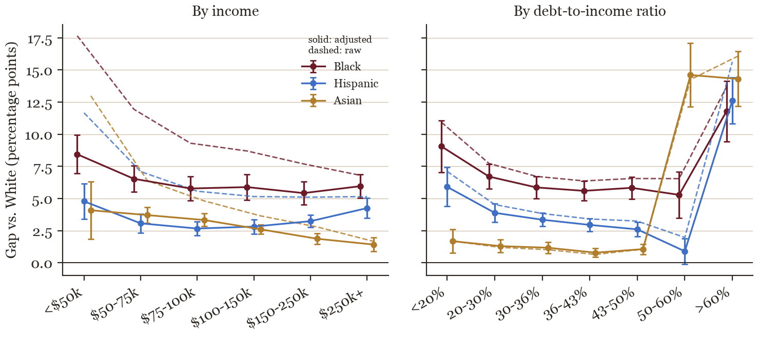
To let the adjusted gap differ by band, we add to model (3) interactions of the Black, Hispanic and Asian indicators with six income bands, and separately with seven debt-to-income bands, and compute \(\hat \Delta _g\) over the group’s applications in each band (Figure 3 and Tables 7 and 8). The raw Black–White gap falls steeply with income, from 17.7 points below $50,000 to 6.8 above $250,000, because low-income applications are denied more often in every group (15.7% of White applications below $50,000). The adjusted gap falls much less, from 8.4 to 6.0: Black applicants earning over $250,000 were denied 11.4% of the time.
| Band | Black raw | adjusted | Hispanic raw | adjusted | Asian raw | adjusted |
| \(<\)$50k | 17.7 | 8.4 (0.77) | 11.7 | 4.8 (0.70) | 13.0 | 4.1 (1.14) |
| $50-75k | 11.9 | 6.5 (0.52) | 7.1 | 3.1 (0.37) | 6.4 | 3.7 (0.31) |
| $75-100k | 9.3 | 5.8 (0.48) | 5.6 | 2.7 (0.27) | 4.8 | 3.3 (0.26) |
| $100-150k | 8.7 | 5.9 (0.50) | 5.2 | 2.8 (0.28) | 3.6 | 2.6 (0.18) |
| $150-250k | 7.7 | 5.4 (0.45) | 5.1 | 3.2 (0.24) | 2.8 | 1.9 (0.21) |
| $250k+ | 6.8 | 6.0 (0.47) | 5.2 | 4.2 (0.40) | 1.7 | 1.4 (0.27) |
| Band | Black raw | adjusted | Hispanic raw | adjusted | Asian raw | adjusted |
| \(<\)20% | 10.9 | 9.1 (1.04) | 7.1 | 5.9 (0.77) | 1.7 | 1.7 (0.47) |
| 20-30% | 7.7 | 6.7 (0.48) | 4.5 | 3.9 (0.37) | 1.2 | 1.3 (0.25) |
| 30-36% | 6.7 | 5.9 (0.44) | 3.8 | 3.3 (0.26) | 1.0 | 1.2 (0.22) |
| 36-43% | 6.4 | 5.6 (0.39) | 3.4 | 2.9 (0.26) | 0.6 | 0.8 (0.18) |
| 43-50% | 6.6 | 5.8 (0.44) | 3.2 | 2.6 (0.28) | 1.1 | 1.1 (0.21) |
| 50-60% | 6.5 | 5.3 (0.91) | 2.0 | 0.9 (0.51) | 14.3 | 14.6 (1.26) |
| \(>\)60% | 13.7 | 11.8 (1.20) | 15.6 | 12.6 (0.91) | 16.1 | 14.3 (1.09) |
Across debt-to-income bands the Black and Hispanic adjusted gaps are largest below 20%, change little between 20 and 50%, and widen again in the top band, where most applications are denied (72.5% of White and 86.2% of Black applications with a ratio above 60%). The Asian pattern is different and, to us, unexpected: a raw gap of 0.6 points at ratios of 36–43%, then 14.6 points (adjusted) at 50–60%, where 28.1% of 11,887 Asian applications were denied against 13.9% of White ones. The gap is not confined to one lender, and the debt-to-income ratio is the reason most often cited. A plausible guess is that something about how income is documented or counted near the 50% threshold differs, but the public data cannot say what, and we report the pattern without an explanation.
4.4 Across states
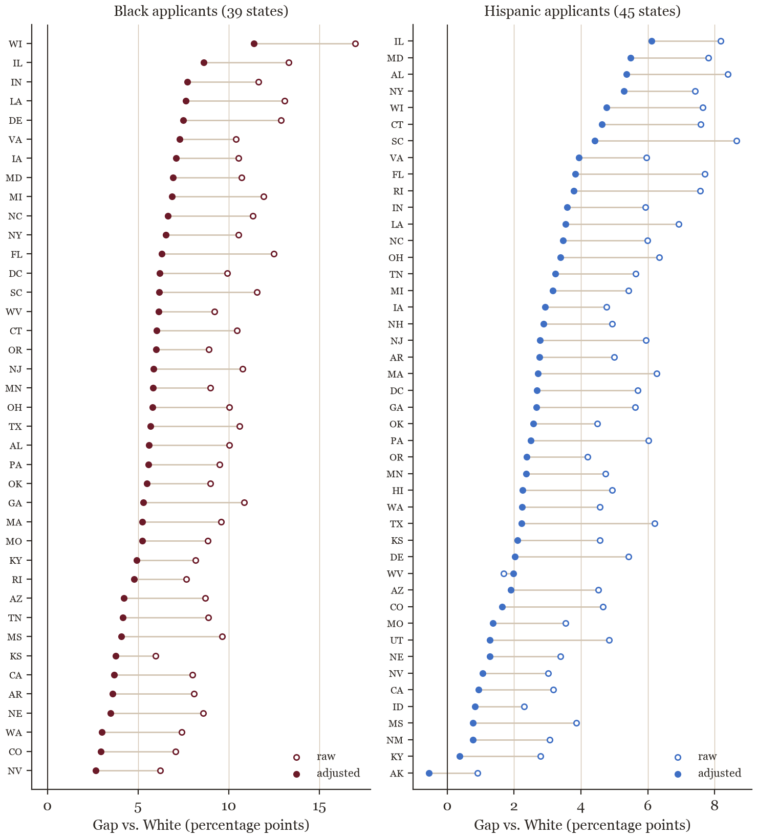
Figure 4 shows, for each state with at least 300 applications in both groups, the raw gap and the adjusted gap \(E_g - E_W\) computed within the state. The adjusted Black–White gap is positive in 39 of the 39 such states, from 2.7 (NV) to 11.4 (WI) points (median 5.8). The adjusted Hispanic–White gap is positive in 44 of 45 states, from -0.6 (AK) to 6.1 (IL) (median 2.7).
4.5 Within lenders
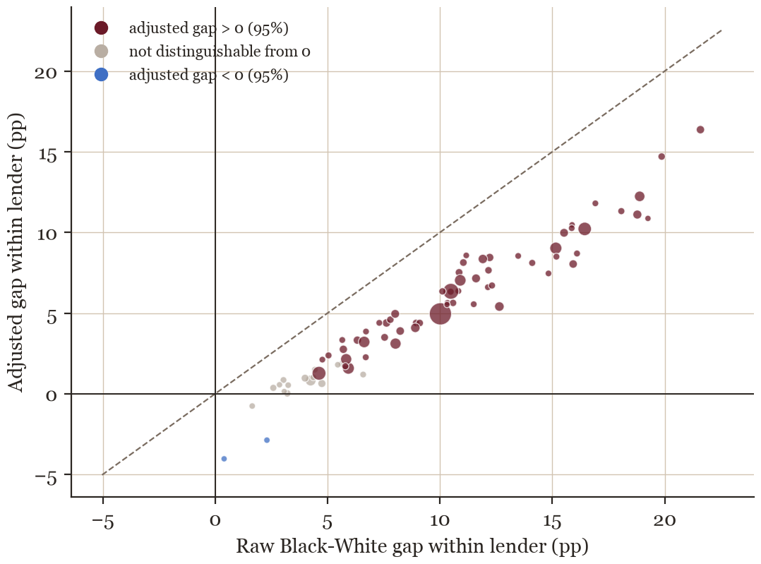
The same decomposition applies to a single lender. For the 77 lenders with at least 500 Black and 500 White applications (together 59.3% of all complete cases), Figure 5 plots the raw Black–White gap within the lender against the adjusted gap \(E_B - E_W\) computed on that lender’s applications. All 77 have a positive raw gap (median 9.1 points). The adjusted gaps are smaller (median 5.0, interquartile range 1.9 to 8.1); 60 are positive at the 5% level by the benchmark standard error and 2 are significantly negative. Because that standard error understates the uncertainty, these counts overstate how many lender-level gaps are distinguishable from zero. We do not name the lenders: an adjusted gap is not a finding of discrimination, for the reasons in Section 5.
4.6 Reasons for denial
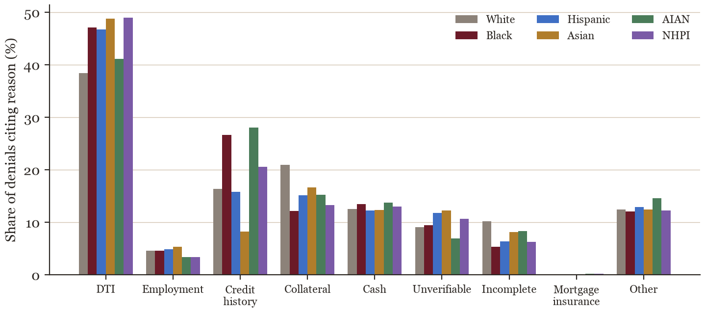
Lenders report up to four reasons for each denial; all 234,667 denials in the complete cases carry at least one. Table 9 and Figure 6 give the share of denials citing each reason. The debt-to-income ratio is the most common reason for every group, and more common for minority applicants (47% of Black and 47% of Hispanic denials, against 38% of White). Credit history is cited in 27% of Black denials and 28% of AIAN denials, against 16% of White and 8% of Asian denials, while collateral is cited more often for White applicants (21%, against 12% for Black). Credit history is exactly what the public data do not record, and its prominence among Black denials is a direct sign that the omitted credit score is likely to matter. The reasons are the lender’s own account, however, and are not audited.
| Reason cited | White | Black | Hispanic | Asian | AIAN | NHPI |
| Debt-to-income ratio | 38% | 47% | 47% | 49% | 41% | 49% |
| Employment history | 5% | 5% | 5% | 5% | 3% | 3% |
| Credit history | 16% | 27% | 16% | 8% | 28% | 21% |
| Collateral | 21% | 12% | 15% | 17% | 15% | 13% |
| Insufficient cash | 13% | 14% | 12% | 12% | 14% | 13% |
| Unverifiable information | 9% | 9% | 12% | 12% | 7% | 11% |
| Application incomplete | 10% | 5% | 6% | 8% | 8% | 6% |
| Mortgage insurance denied | 0% | 0% | 0% | 0% | 0% | 0% |
| Other | 12% | 12% | 13% | 12% | 15% | 12% |
| Denials with a reason | 85,726 | 34,290 | 49,102 | 16,187 | 939 | 384 |
5 Limitations
The credit score. The public data omit the credit score [4], and by Proposition 3.8 an omitted variable that raises denial and differs by group biases the adjusted gap in its direction. With the confidential HMDA fields, including credit scores and automated underwriting recommendations, Bhutta, Hizmo and Ringo [2] find residual gaps of 1 to 2 percentage points and evidence that unobserved risk explains at least part of those. Our adjusted gaps are larger, which is what one would expect if much of the remainder is credit risk that the public data do not show; but their sample, years and methods differ from ours, so the comparison is suggestive only.
Coarse controls. Income, loan amounts, property values and ages are rounded or binned in the public file, and the debt-to-income ratio is binned outside 36–49%. Within a bin, groups may differ systematically; such differences are omitted variables too.
Selection. We see only those who applied, and only applications that reached a decision. Applicants who expect to be denied may not apply, may withdraw, or may go to a different lender or loan type, and differences in who applies change the meaning of a denial rate. The complete-case restriction drops 5.3% of applications, disproportionately denials.
Controls that may carry the disparity. Some controls may themselves reflect unequal treatment: the loan type an applicant ends up with, the lender they apply to, or the appraised value. Holding them fixed can understate a disparity, which is one reason we show the whole ladder rather than a single number.
Discrimination is a legal question. Fair-lending law distinguishes disparate treatment from disparate impact, and what counts as a legitimate business justification is a legal judgement [7, 9]. A statistical gap, adjusted or not, is evidence for that judgement, not the judgement itself. Disparities can also arise in the price of credit rather than its approval: Bartlett, Morse, Stanton and Wallace [1] find that risk-equivalent Latinx and Black borrowers paid higher interest rates on GSE-securitized and FHA-insured loans.
Uncertainty. Model standard errors are clustered by lender. The benchmark standard errors used for states, lenders and the explorer are binomial and ignore both clustering and the estimation of the benchmark; they are too small.
6 Conclusion
In 2025, Black applicants for a home-purchase mortgage were denied 16.7% of the time and White applicants 5.9%. What the public HMDA data record about the applicant, the loan, the property and the state accounts for 42% of that gap, and comparing applicants at the same lender in the same county leaves 4.4 percentage points. Hispanic, Asian, AIAN and NHPI applicants show smaller adjusted gaps (3.1, 2.3, 2.2 and 2.9 points in model (3)). The adjusted Black–White gap is positive in every state we can measure and at nearly every large lender, and it narrows only a little as income rises. Whether that remainder is credit risk that the public data cannot see, unequal treatment, or both is a question these data cannot settle; research with the credit score suggests that a large part of it may be the former. The explorer at https://maths.dsmorgan.com/projects/mortgage-denials/explore lets the reader repeat these comparisons for a state, an income or debt-to-income band, or a loan type.
References
- [1]
- R. Bartlett, A. Morse, R. Stanton and N. Wallace, Consumer-lending discrimination in the FinTech era, Journal of Financial Economics 143(1) (2022), 30–56, https://doi.org/10.1016/j.jfineco.2021.05.047.
- [2]
- N. Bhutta, A. Hizmo and D. Ringo, How much does racial bias affect mortgage lending? Evidence from human and algorithmic credit decisions, Journal of Finance 80(3) (2025), 1463–1496, https://doi.org/10.1111/jofi.13444. Earlier version: Finance and Economics Discussion Series 2022-067, Board of Governors of the Federal Reserve System, https://doi.org/10.17016/FEDS.2022.067.
- [3]
- Consumer Financial Protection Bureau, Home Mortgage Disclosure (Regulation C), final rule, 80 Fed. Reg. 66128 (28 October 2015); Regulation C is codified at 12 CFR part 1003.
- [4]
- Consumer Financial Protection Bureau, Disclosure of loan-level HMDA data, final policy guidance, 84 Fed. Reg. 649 (31 January 2019).
- [5]
- Federal Financial Institutions Examination Council, Public HMDA – LAR Data Fields, https://ffiec.cfpb.gov/documentation/publications/loan-level-datasets/lar-data-fields; 2025 Snapshot National Loan-Level Dataset, https://ffiec.cfpb.gov/data-publication/snapshot-national-loan-level-dataset/2025.
- [6]
- Consumer Financial Protection Bureau, HMDA platform documentation, Derived fields categorization, 2018 onward, https://github.com/cfpb/hmda-platform/wiki/Derived-Fields-Categorization-2018-Onward.
- [7]
- H. F. Ladd, Evidence on discrimination in mortgage lending, Journal of Economic Perspectives 12(2) (1998), 41–62, https://doi.org/10.1257/jep.12.2.41.
- [8]
- A. H. Munnell, G. M. B. Tootell, L. E. Browne and J. McEneaney, Mortgage lending in Boston: interpreting HMDA data, American Economic Review 86(1) (1996), 25–53.
- [9]
- S. L. Ross and J. Yinger, The Color of Credit: Mortgage Discrimination, Research Methodology, and Fair-Lending Enforcement, MIT Press, 2002.